Three-dimensional full-field X-ray orientation microscopy in tomosipo

Oct 2, 2020

Allard Hendriksen

9 minute read

Goal

This blog post is written to evaluate the possibility of including the geometry described in (Viganò et al. 2016) in a future paper about tomosipo.

The first goal is to check whether I have correctly understood the concepts in the cited paper.
The second goal is to examine how to efficiently describe this geometry using tomosipo.

Introduction

Conventional X-ray absorption tomography can be used to determine the density of the interior of an object. In addition to the density, it is often useful to know the orientation of sub-volumes of the interior of an object, for instance to discover the grain structure of a crystalline object, such as a metal composite. Near-field X-ray diffraction tomography can be used to determine the orientation of volume elements at a very high resolution. In this blog post, we describe a recently published approach (Viganò et al. 2016).

Absorption tomography

In conventional X-ray absorption tomography, an object rotates around an axis in front of a planar detector. X-rays penetrate the object, and move along rays that are orthogonal to the detector. As the rays move through the object, their brightness is attenuated by the object. This is displayed below.

import tomosipo as ts
from tomosipo.qt import animate
import numpy as np

# Create a volume and a planar parallel-beam detector
vg = ts.volume(pos=(0, -1, 0)).to_vec()
pg = ts.parallel(angles=1, shape=2).to_vec()

# Rotate the volume around its center
angles = np.linspace(0, np.pi, 20)
R = ts.rotate(pos=vg.pos, axis=(1, 0, 0), rad=angles)

# Scale and rotate to obtain a pleasant viewing angle
V = ts.scale(2) * ts.rotate(pos=0, axis=(1, 0, 0), deg=75)

animate(V * R * vg, V * pg)

Bragg reflection

Crystals are arranged in a lattice structure. Due to this structure, and wave interference of light, crystals diffract X-rays. This effect is described by Bragg’s law and is defined as a reflection in the plane of the crystal lattice. The illustration below describes how a pencil beam is reflected in the lattice plane of a crystal. In the code below, the definition of reflect is omitted; it is included at the bottom of this post.

# Create a thin pencil beam and a detector
beam = ts.volume(size=(0.01, 5, 0.01)).to_vec()
detector = ts.volume(pos=(0, 2, 0), size=(4, 0.01, 4)).to_vec()

# Create some basic elements
ground_plane = ts.volume(pos=0, size=(0.01, 1, 1)).to_vec()
z_axis = ts.volume(pos=ground_plane.pos, size=(1, 0.01, 0.01)).to_vec()

# Create a crystal volume element.
# Write the orientation as a small rotation
crystal_O = ts.rotate(pos=0, axis=(0.0, 1.0, 1.0), rad=0.3)
# Rotate the ground plane and z-axis to obtain the oriented crystal plane
# and normal vector
crystal_plane = crystal_O * ground_plane
crystal_normal = crystal_O * z_axis

# Create a mirror symmetry in the crystal plane
M = reflect(pos=crystal_plane.pos, axis=crystal_plane.w)
reflected_beam = M * beam

# Scale and rotate to obtain a pleasant viewing angle
V = ts.translate((0, -1, 0.5))
V = ts.rotate(pos=0, axis=(1, 0, 0), deg=75) * V
V = ts.scale(1.5) * V

animate(
    V * beam,
    V * detector,
    V * crystal_plane,
    V * crystal_normal,
    V * reflected_beam
)

Diffraction tomography

When the sample is rotated, the diffracted beam leaves a trace on the detector. This information can be used to determine the orientation of the crystal lattice in different parts of the sample.

# Create a rotation operator around the Z axis
angles = np.linspace(0, 2 * np.pi, 50)
R = ts.rotate(pos=0, axis=(1, 0, 0), rad=angles)

# Create a rotation axis, and the rotated plane, and normal
# vector for display
rot_axis = ts.volume(pos=0, size=(5, 0.01, 0.01)).to_vec()
rotated_plane = R * crystal_plane
rotated_normal = R * crystal_normal

# Create a mirror symmetry in the rotated_plane
M = reflect(pos=rotated_plane.pos, axis=rotated_plane.w)
diffracted_beam = M * beam

animate(
    V * beam,
    V * detector,
    V * rot_axis,
    V * rotated_plane,
    V * rotated_normal,
    V * diffracted_beam,
)

In fact, in the approach described (Viganò et al. 2016), the orientation space is split into a regular grid containing small scattering angles. The animation below rotates the normal vectors of these orientations:

z, y, x = np.array([[1, 0, 0], [0, 1, 0], [0, 0, 1]])
angular_range = np.pi / 20
steps = 3
diffraction_angles = np.linspace(-angular_range, angular_range, steps, endpoint=True)

diff_normal = z
# O is a sequence of rotations in orientation space
Oy = ts.concatenate([ts.rotate(pos=0, axis=y, rad=a) for a in diffraction_angles])
Ox = ts.concatenate([ts.rotate(pos=0, axis=x, rad=a) for a in diffraction_angles])
O = ts.concatenate([oy * ox for oy in Oy for ox in Ox])

# Display all orientations and rotate them:
animate(*(ts.scale(1.5) * R * o * z_axis for o in O))

For a single lattice orientation, we can describe the physical image formation process due to diffraction with an ASTRA geometry. When we assume that absorption in the sample is negligible, then the signal due to diffraction can be projected onto the detector by altering the ray direction in the ASTRA geometry. This is described below for the first lattice orientation.

## These functions should be included in tomosipo
def transform_vec(T, v):
    hv = vc.to_homogeneous_vec(v)
    return vc.to_vec(vc.matrix_transform(T.matrix, hv))

def transform_point(T, p):
    hp = vc.to_homogeneous_point(p)
    return vc.to_vec(vc.matrix_transform(T.matrix, hp))

# Create a volume centered on the origin and a small detector
# right behind it
vg = ts.volume(size=1, shape=256).to_vec()
T_pg = ts.translate((0, 2, 0))
pg = T_pg * ts.parallel(angles=1, size=4, shape=1024).to_vec()

# For the first orientation in orientation space, create
# a reflection operator.
M = reflect(pos=0, axis=(R * O[0] * z_axis).w)
# Create similarly sized identity transform.
I = ts.concatenate([ts.geometry.transform.identity() for _ in R])

# Create a projection where the ray direction follows the
# reflected beam, and other parameters are unchanged.
oriented_pg = ts.parallel_vec(
    shape=pg.det_shape,
    ray_dir=transform_vec(M, pg.ray_dir),
    det_pos=transform_point(I,  pg.det_pos),
    det_v=transform_point(I, pg.det_v),
    det_u=transform_point(I, pg.det_u),
)

# Show result:
beam = ts.volume(size=(0.01, 5, 0.01)).to_vec()
z_axis = ts.volume(pos=ground_plane.pos, size=(5, 0.01, 0.01)).to_vec()
animate(
    V * R * vg,
    V * oriented_pg,
    V * R * O[0] * z_axis,
    V * M * beam,
    V * beam,
)

Equivalently, we can rotate the projection geometry instead of rotating the volume:

animate(vg, R.inv * oriented_pg)

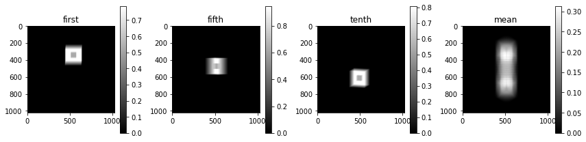
Forward projection

Using this geometry, we can create a forward projection operator for the first orientation. We use this operator to forward project a hollow cube phantom.

import matplotlib.pyplot as plt

# Forward operator
A = ts.operator(vg, R.inv * oriented_pg)

# Create a hollow cube phantom
x = np.zeros(A.domain_shape, dtype=np.float32)
x[32:-32, 32:-32, 32:-32] = 1.0
x[96:-96, 96:-96, 96:-96] = 0.0

# Forward project
y = A(x)

# plot_imgs is defined at the end of the blog post
plot_imgs(
    first=y[:, 0],
    fifth=y[:, 5],
    tenth=y[:, 10],
    mean=y.mean(axis=1),
)

How would the computational code look like?

When computing a reconstruction, pretty animations of the geometry count for nothing. We just need an efficient description of the geometry.

I attempt to describe the full geometry from scratch below.

import tomosipo as ts
from tomosipo.qt import animate
import numpy as np

# axes
z, y, x = np.array([[1, 0, 0], [0, 1, 0], [0, 0, 1]])
###############################################################################
#                              Utility functions                              #
###############################################################################
# These will be included in tomosipo in short order
def transform_vec(T, v):
    hv = vc.to_homogeneous_vec(v)
    return vc.to_vec(vc.matrix_transform(T.matrix, hv))

def transform_point(T, p):
    hp = vc.to_homogeneous_point(p)
    return vc.to_vec(vc.matrix_transform(T.matrix, hp))

###############################################################################
#                                  Parameters                                 #
###############################################################################
# Orientation space
angular_range = np.pi / 20
steps = 3
diffraction_angles = np.linspace(-angular_range, angular_range, steps, endpoint=True)

# Rotation around z-axis
angles = np.linspace(0, np.pi, 40)

# Volume
vol_size = 1
vol_shape = 256 # cubed

# Detector
det_shape = 1024
det_size = 4
det_obj_dist = 2  # Distance between object center and detector

###############################################################################
#                                  Transforms                                 #
###############################################################################
Oy = ts.concatenate([ts.rotate(pos=0, axis=y, rad=a) for a in diffraction_angles])
Ox = ts.concatenate([ts.rotate(pos=0, axis=x, rad=a) for a in diffraction_angles])
O = ts.concatenate([oy * ox for oy in Oy for ox in Ox])

# Create a rotation operator around the Z axis
R = ts.rotate(pos=0, axis=(1, 0, 0), rad=angles)

def create_operator(vg, pg, R, orientation):
    vg, pg = vg.to_vec(), pg.to_vec()
    z_axis = ts.volume(size=(1, 0, 0)).to_vec()
    # Create operator that reflects in the orientation plane.
    M = reflect(pos=0, axis=(R * orientation * z_axis).w)
    # Create similarly sized identity transform.
    I = ts.concatenate([ts.geometry.transform.identity() for _ in M])

    # Create a projection geometry where the ray direction is
    # parallel the reflected beam, and other parameters are
    # unchanged.
    oriented_pg = ts.parallel_vec(
        shape=pg.det_shape,
        ray_dir=transform_vec(M, pg.ray_dir),
        det_pos=transform_point(I,  pg.det_pos),
        det_v=transform_point(I, pg.det_v),
        det_u=transform_point(I, pg.det_u),
    )

    return ts.operator(vg, R.inv * oriented_pg)

###############################################################################
#                   Create volume and detector and operators                  #
###############################################################################
# Create volume and (single-angle) projection geometry on the origin
vg = ts.volume(size=vol_size, shape=vol_shape)
pg = ts.parallel(angles=1, size=det_size, shape=det_shape)
# Move detector away from the origin
T_pg = ts.translate((0, det_obj_dist, 0))
pg = T_pg * pg.to_vec()

operators = [create_operator(vg, pg, R, o) for o in O]

###############################################################################
#                       Forward and backward projection                       #
###############################################################################

# The domain is of shape
# (num_orientations, vol_shape[0], ..., vol_shape[2])
x_shape = (len(operators), *operators[0].domain_shape)
x = np.zeros(x_shape, dtype=np.float32)

# We can describe the forward and backprojection operators as follows
def forward(operators, x):
    y = np.zeros(operators[0].range_shape, dtype=np.float32)
    for A in operators:
        y += A(x)

    return y

def backward(operators, y):
    x_shape = (len(operators), *operators[0].domain_shape)
    x = np.empty(x_shape, dtype=np.float32)

    for A, x_oriented in zip(operators, x):
        A.T(y, out=x_oriented)

    return x

# That was it.

Questions

In the code example above, the non-diffracted (absorption) signal interferes with the diffracted signal.
- Are the scattering angles usually chosen to be larger?
- Or is the detector larger?
- Or is the detector placed further away?
Is the assumption that absorption is negligible correct? The paper states “Assuming kinematic diffraction and neglecting photoelectric absorption and extinction effect”.
Is the description of Bragg reflection approximately correct?

Omitted code

I am planning to include the following piece of code in the tomosipo package, since reflection is a fundamental geometric transform.

from tomosipo.geometry.transform import identity, Transform
from tomosipo import vector_calc as vc

def reflect(pos, axis):
    """Reflect in the plane through `pos` with normal vector `axis`

    The parameters `pos` and `axis` are interpreted as
    homogeneous coordinates. You may pass in both homogeneous or
    non-homogeneous coordinates. Also, you may pass in multiple rows
    for multiple timesteps. The following shapes are allowed:

    - `(n_rows, 3)` [non-homogeneous] or `(n_rows, 4)` [homogeneous]
    - `(3,)` [non-homogeneous] or `(4,)` [homogeneous]

    :param pos: `np.array` or `scalar`
        A position intersecting the plane of reflection.
    :param axis:
        A normal vector to the plane of reflection. Need not be unit-normal.

    :returns:
    :rtype:

    """
    if np.isscalar(pos):
        pos = ts.utils.to_pos(pos)
    pos = vc.to_homogeneous_point(pos)
    axis = vc.to_homogeneous_vec(axis)
    pos, axis = vc._broadcastv(pos, axis)
    axis = axis / vc.norm(axis)[:, None]

    # Create a householder matrix for reflection through the origin.
    # https://en.wikipedia.org/wiki/Householder_transformation
    R_origin = ts.concatenate([
        Transform(identity().matrix - 2 * np.outer(a, a))
        for a in axis
    ])

    T = ts.translate(pos)

    return T * R_origin * T.inv

I use this helper function to display multiple images:


def plot_imgs(height=3, cmap="gray", clim=(None, None), **kwargs):
    fig, axes = plt.subplots(
        nrows=1,
        ncols=len(kwargs),
        figsize=(height * len(kwargs), height)
    )
    if len(kwargs) == 1:
        axes = [axes]
    for ax, (k, v) in zip(axes, kwargs.items()):
        pcm = ax.imshow(v.squeeze(), cmap=cmap, clim=clim)
        fig.colorbar(pcm, ax=ax)
        ax.set_title(k)
    fig.tight_layout()

Bibliography

Viganò, Nicola, Alexandre Tanguy, Simon Hallais, Alexandre Dimanov, Michel Bornert, Kees Joost Batenburg, and Wolfgang Ludwig. 2016. “Three-Dimensional Full-Field X-Ray Orientation Microscopy. S/c”ientific Reports/ 6 (1). Nature Publishing Group:1–9.

Allard Hendriksen | CI @ CWI