Allard Hendriksen | CI @ CWI

Is it possible to write a custom CUDA kernel that outperforms the standard convolution operator in PyTorch?

For historical reasons, I have implemented custom convolutions using CUDA for use in PyTorch. These convolutions allowed my to work around PyTorch limitations regarding memory safety, leading to an efficient implementation of the Mixed-scale dense network architecture (Pelt and Sethian 2017). Recently, a user asked why I had implemented these convolutions. To answer that question, I decided to benchmark and compare my custom implementation to the standard convolutions in PyTorch.

The convolutions in PyTorch are executed by Nvidia’s cuDNN library, which is heavily optimized. Nonetheless, in the cuDNN paper (Chetlur et al. 2014), the authors hint at one possible approach to improve performance beyond what is possible cuDNN:

Another common approach is to compute the convolutions directly. This can be very efficient, but requires a large number of specialized implementations to handle the many corner cases implicit in the 11-dimensional parameter space of the convolutions. Implementations following this approach are often well-optimized for convolutions in certain parts of the parameter space, but perform poorly for others.

Let’s find out if I succeeded!

How to determine execution speed?

To determine the execution times, we will use an approach that is specifically designed to measure very small execution times (Moreno and Fischmeister 2017). This approach enables getting accurate statistics for the execution time of a function. The trick is to execute the function a variable number of times, while keeping the benchmark setup code constant. Then a linear regression can be performed on the running times to determine the time that a single execution of the function takes.

As an example, let’s determine the time that it takes to sort an array of 100,000 already ordered values in NumPy. This code is inspired by the excellent example code by Bernard Knasmueller.

import numpy as np
import matplotlib.pyplot as plt
from time import perf_counter as timer


def iter_np_sort(num_iters):
    # Setup of problem
    # Constant time (to be ignored)
    x = np.arange(100_000)

    # Run function
    # Variable time (variable of interest)
    for _ in range(num_iters):
        _ = np.sort(x)


def timeit(f, it):
    start = timer()
    f(it)
    return timer() - start

num_trials = 10
num_iters = np.array([0, 1, 2, 3, 4, 5] * num_trials)
execution_times = np.array([timeit(iter_np_sort, it) for it in num_iters])

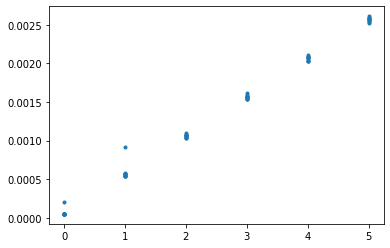
plt.plot(num_iters, execution_times, '.')
plt.show()

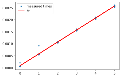
The slope of this graph is determined by the time it takes to sort an array once.

slope, intercept = np.polyfit(num_iters, execution_times, deg=1)

print(f"Intercept: {intercept: 0.2e} seconds (time to set the problem up)")
print(f"Slope:     {slope: 0.2e} seconds (time to sort)")

Intercept:  7.40e-05 seconds (time to set the problem up)
Slope:      4.98e-04 seconds (time to sort)

As you can see below, the fit is pretty good.

plt.plot(num_iters, execution_times, '.', label="measured times")
plt.plot(num_iters, slope * num_iters + intercept, 'r', label="fit")
plt.legend()
plt.show()

With some additional work, you can also derive confidence intervals for the variance of the execution time. The code to do this is attached at the end of this post.

Custom convolutions

We test the time it takes to execute a convolution and ReLU operation. We use the following code to execute the custom convolutions and the PyTorch-provided convolutions.

import torch
import matplotlib.pyplot as plt
from functools import partial
from msd_pytorch.conv_relu import ConvRelu2dInPlaceFunction

custom_conv = ConvRelu2dInPlaceFunction.apply

def iter_conv(iterations, c_in=1, c_out=1, N=32, dilation=1, use_torch=False, backward=True):
    # Create input, weight, and bias        (constant time)
    x = torch.randn(1, c_in, N, N).cuda()
    w = torch.randn(c_out, c_in, 3, 3, requires_grad=True).cuda()
    bias = torch.randn(c_out, requires_grad=True).cuda()
    # Perform convolution                   (variable time)
    for _ in range(iterations):
        if use_torch:  # PyTorch convolution
            y = torch.conv2d(x, w, bias, padding=dilation, dilation=dilation)
            y = torch.nn.functional.relu(y)
        else:          # Our custom convolution
            # We need to preallocate y (part of variable execution time)
            y = torch.empty(1, c_out, N, N, device='cuda')
            y = custom_conv(x, w, bias, y, 1, dilation)

        if backward:
            y.backward(torch.ones_like(y))
        torch.cuda.synchronize()

Benchmarks

We measure the execution time for various image sizes, and plot the result.

# Vary image size:
Ns = 2 ** np.arange(3, 10)

plt.title("Execution time")
for use_torch in [True, False]:
        timings = [
            measure_small_execution_time(
                partial(iter_conv, N=N, c_in=1, c_out=1, dilation=1, use_torch=use_torch),
                num_trials=20,
            ) for N in Ns
        ]

        plot_timings(
            Ns, timings,
            label="Torch forward+backward" if use_torch else "Custom forward+backward",
            color="r" if use_torch else "b",
        )
plt.xlabel("Image size (N x N)")
plt.ylabel("Time (s)")
plt.ylim((0, None))
plt.legend()
plt.show()

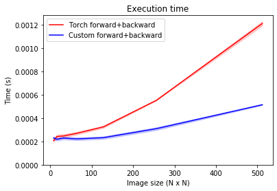
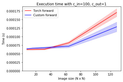
As you can see, our custom convolution implementation is consistently faster, especially as the size of the image increases. This plot is relevant for training, where the backward pass is executed to determine the parameter updates. When executing a trained network on new data, only the forward pass is executed, which we benchmark below.

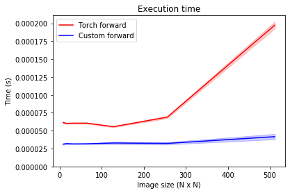
Here, the same thrend is visible. Note that the forward pass is significantly faster than the backward pass, so this difference might not be as relevant in practice.

Coming back to square one

The previous results suggest that the custom convolution code is substantially faster than cuDNN. This is not the case for all inputs though. CuDNN is very optimized for cases where the number of input and output channels of the convolution is relatively large. So far, the number of input and output channels has been fixed at one.

When we fix the image size, and vary the number of input and output channels, the results are different. As shown below, when the the number of input and output channels is equal and increases, the PyTorch convolutions are substantially faster. To a lesser extent, this effect is also present when the number of output channels is kept constant and the number of input channels increases quadratically. Curiously, with a single input channel, the performance is the same.

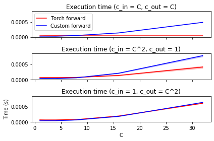
These results seem to corroborate the statement in the cuDNN paper that custom implementations may be faster for in some cases, but probably not in every case.

At larger image sizes, however, cuDNN loses its edge again. When the number of output channels is small, the custom implementation is relatively faster again.

Conclusion

If you have a specific use case, you may very well be able to write a custom convolution kernel that is faster than the kernel provided by cuDNN. In the case of the mixed-scale dense network architecture, the number of output channels frequently equals one. Hence, these custom convolutions provide a nice speed-up compared to the standard PyTorch convolutions.

The second question is whether you should write a custom convolution kernel. That answer is probably no. Supporting custom CUDA and C++ code across versions of PyTorch and Python is a major pain in the ass. In the case of msd_pytorch, just publishing a new version of the package can take up to eight hours, because of the large matrix of targets, slow compile times, and Docker inefficiencies. For this package, however, there are other very good reasons to not use the standard convolutions. I might write about that at some point in the future.

Appendix

This is the code that is used to estimate the execution times, and the confidence intervals.

import torch
import numpy as np
import matplotlib.pyplot as plt
from functools import partial


def timeit(f, it):
    torch.cuda.synchronize()
    start = timer()
    f(it)
    torch.cuda.synchronize()
    return timer() - start

def measure_small_execution_time(f,
                                 num_iters=[0,1,2,3],
                                 num_trials=2,
                                 ci=True):
    """Measures the execution time of a function f

    `f` must take an int `it` and compute `it` iterations.

    This function estimates how long a single iteration works using the
    methodology proposed in

    Moreno, C., & Fischmeister, S. (2017). Accurate measurement of small
    execution times—getting around measurement errors. IEEE Embedded Systems
    Letters, 9(1), 17–20. http://dx.doi.org/10.1109/les.2017.2654160

    The function returns:
    1. an estimate for the execution time of a single iteration, and
    2. a 90% confidence interval for the estimate (if `ci=True`).

    """
    # Warmup
    f(max(num_iters))
    # Measure
    num_iters = np.array(list(num_iters) * num_trials)
    timings = np.array([timeit(f, it) for it in num_iters])

    slope, intercept = np.polyfit(num_iters, timings, deg=1)

    if not ci:
        return slope

    # Follows exposition in:
    # https://en.wikipedia.org/wiki/Simple_linear_regression#Confidence_intervals
    n = len(timings)
    timings_hat = slope * num_iters + intercept
    error = timings_hat - timings
    s_beta_hat = np.sqrt(
        1 / (n - 2) * np.sum(error ** 2) /
        np.sum((num_iters - num_iters.mean()) ** 2)
    )
    # Sample a million elements form a standard_t distribution for 90%
    # confidence interval
    N = 1_000_000
    t = np.sort(np.random.standard_t(n - 2, N))
    ci_5, ci_95 = t[5 * N // 100], t[95 * N // 100]

    ci = (slope + ci_5 * s_beta_hat, slope + ci_95 * s_beta_hat)
    return slope, ci

def plot_timings(x, timings, label=None, color="blue", linestyle="-", ci=True, ax=None):
    if ax is None:
        ax = plt
    if ci:
        timings_estimate = np.array([t[0] for t in timings])
        timings_ci_min = np.array([t[1][0] for t in timings])
        timings_ci_max = np.array([t[1][1] for t in timings])
    else:
        timings_estimate = np.array(timings)

    ax.plot(x, timings_estimate, linestyle=linestyle, color=color, label=label)
    if ci:
        ax.fill_between(x, timings_ci_min, timings_ci_max, color=color, alpha=0.2)

Bibliography

Chetlur, Sharan, Cliff Woolley, Philippe Vandermersch, Jonathan Cohen, John Tran, Bryan Catanzaro, and Evan Shelhamer. 2014. “cuDNN: Efficient Primitives for Deep Learning. C/o”RR/. http://arxiv.org/abs/1410.0759v3.

Moreno, Carlos, and Sebastian Fischmeister. 2017. “Accurate Measurement of Small Execution Times—Getting Around Measurement Errors. I/E”EE Embedded Systems Letters/ 9 (1). Institute of Electrical and Electronics Engineers (IEEE):17–20. http://dx.doi.org/10.1109/LES.2017.2654160.

Pelt, Daniël M., and James A. Sethian. 2017. “A Mixed-Scale Dense Convolutional Neural Network for Image Analysis. P/r”oceedings of the National Academy of Sciences/ 115 (2). Proceedings of the National Academy of Sciences:254–59. https://doi.org/10.1073/pnas.1715832114.