Advent of tomosipo: s003_gpu_reconstruction
Today, we are going to reconstruct on the GPU. This is a great example, because it allows us to play around with PyTorch on the GPU to improve performance.
Geometries
First, we define the same geometries we had before:
import astra
import tomosipo as ts
import numpy as np

# Create ASTRA geometries
vol_geom = astra.create_vol_geom(256, 256)
angles = np.linspace(0, np.pi, 180, False)
proj_geom = astra.create_proj_geom('parallel', 1.0, 384, angles)
# Create tomosipo geometries
vg = ts.volume(shape=(1, 256, 256))
pg = ts.parallel(angles=180, shape=(1, 384))
A = ts.operator(vg, pg)
Sinogram
We generate a sinogram, like we did in the first installment. We use the
domain_shape property of the operator we defined in the code block above to
determine the shape of the data.
# Slightly off-center hollow box phantom
phantom = np.zeros(A.domain_shape, dtype=np.float32)
phantom[:, 42:234, 42:234] = 1.0  # box
phantom[:, 74:202, 74:202] = 0.0  # and hollow

# Generate sinogram using ASTRA
proj_id = astra.create_projector('cuda',proj_geom,vol_geom)
sinogram_id, sinogram = astra.create_sino(phantom[0], proj_id)

# Generate sinogram using tomosipo
sino = A(phantom)
Reconstruction
ASTRA has some pre-installed reconstruction algorithms you can use:
# Create a data object for the reconstruction
rec_id = astra.data2d.create('-vol', vol_geom)
# Set up the parameters for a reconstruction algorithm using the GPU
cfg = astra.astra_dict('SIRT_CUDA')
cfg['ReconstructionDataId'] = rec_id
cfg['ProjectionDataId'] = sinogram_id

# Create the algorithm object from the configuration structure
alg_id = astra.algorithm.create(cfg)

# Run 150 iterations of the algorithm
num_iterations = 150
astra.algorithm.run(alg_id, num_iterations)

# Get the result
rec = astra.data2d.get(rec_id)
Tomosipo does not contain any reconstruction algorithms, but the SIRT algorithm is quite simple to program yourself. The algorithm is defined by
\begin{align*}
x_0 &= \mathbf{0} \\\
x_{n+1} &= C A^T R (y - A x_n) \\\
\end{align*}
with diagonal matrices \(C\) and \(R\), defined by
\begin{align*}
C_{jj} &= \frac{1}{\sum_{i} a_{ij}}, \\\
R_{ii} &= \frac{1}{\sum_{j} a_{ij}}. \\\
\end{align*}
This is explained in more detail at Tom Roelandt’s blog.
# Prepare preconditioning matrices R and C. Since the matrices are diagonal,
# we use vectors of the same shape as x and y (they multiply element-wise
# in numpy).
R = 1 / A(np.ones(A.domain_shape))
R = np.minimum(R, 1 / ts.epsilon)
C = 1 / A.T(np.ones(A.range_shape))
C = np.minimum(C, 1 / ts.epsilon)

# Reconstruct from sinogram y into x_rec
x_rec = np.zeros(A.domain_shape, dtype=np.float32)

for i in range(num_iterations):
    x_rec += C * A.T(R * (sino - A(x_rec)))
import matplotlib.pyplot as plt


def plot_imgs(height=3, cmap="gray", clim=(None, None), **kwargs):
    fig, axes = plt.subplots(
        nrows=1,
        ncols=len(kwargs),
        figsize=(height * len(kwargs), height)
    )
    if len(kwargs) == 1:
        axes = [axes]
    for ax, (k, v) in zip(axes, kwargs.items()):
        pcm = ax.imshow(v.squeeze(), cmap=cmap, clim=clim)
        fig.colorbar(pcm, ax=ax)
        ax.set_title(k)
    fig.tight_layout()

plot_imgs(**{
    "Phantom\n": phantom[0],
    "Reconstruction\nASTRA": rec,
    "Reconstruction\ntomosipo": x_rec[0],
    "Difference\n": rec-x_rec[0],
})
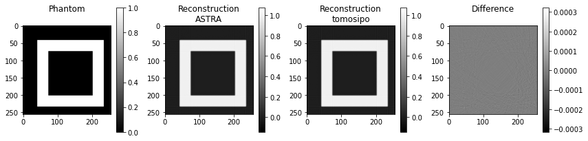
As you can see, there are some minor differences, which are probably caused by numerical rounding errors.
Fast reconstruction
If you are following along in Python, you may have noticed that the SIRT implementation in Numpy was a bit slower than ASTRA’s implementation. This is caused by the fact that ASTRA keeps the data on GPU and performs the multiplication by C and R on the GPU as well. Our implementation, however, has to shuttle the data between GPU and CPU every time an ASTRA operation takes place. ASTRA operates on the GPU and numpy on the CPU.
To overcome this issue, we move all computations to the GPU using PyTorch. If you are unfamiliar with PyTorch, you may find the Pytorch for Numpy users guide useful.
# First, enable pytorch support in tomosipo
import tomosipo.torch_support
# Import torch as well
import torch

y = torch.from_numpy(sino)

# Prepare preconditioning matrices R and C
R = 1 / A(torch.ones(A.domain_shape))
torch.clamp(R, max=1 / ts.epsilon, out=R)
C = 1 / A.T(torch.ones(A.range_shape))
torch.clamp(C, max=1 / ts.epsilon, out=C)

# Reconstruct from sinogram y into x_rec

# NOTE: setting the dtype to float32 explicitly is not necessary for torch.
# The default accuracy is 32 bits.
x_rec = torch.zeros(A.domain_shape)

for i in range(num_iterations):
    x_rec += C * A.T(R * (y - A(x_rec)))
This is nice. It uses PyTorch. It is still slow. PyTorch is not automatically faster than numpy. By default, it processes data on the CPU as well. Therefore, we must move the data to GPU explicitly.
device = torch.device("cuda") # or "cpu"
y = y.to(device)
R = R.to(device)
C = C.to(device)

x_rec = torch.zeros(A.domain_shape, device=device)

for i in range(num_iterations):
    x_rec += C * A.T(R * (y - A(x_rec)))

# And move final result to CPU
x_rec = x_rec.cpu()
# And convert to numpy array for plotting
x_rec = x_rec.numpy()

plot_imgs(
    phantom=phantom,
    pytorc=x_rec[0],
    phantom_diff=x_rec[0]-phantom,
    astra_diff=x_rec[0]-rec,
)
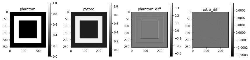
For small data, the difference is not huge in absolute terms. In relative terms, we still obtain a 16% speed-up. This difference grows as the data grows in size. At relatively modest data sizes, the pytorch implementation of SIRT starts to beat ASTRA’s implementation, as can be verified using the SIRT benchmark code.
from timeit import default_timer as timer

for device in ["cpu", "cuda"]:
    start = timer()
    print(f"{device:<10}: ", end="")
    device = torch.device(device)
    y = y.to(device)
    R = R.to(device)
    C = C.to(device)

    x_rec = torch.zeros(A.domain_shape, device=device)

    for i in range(num_iterations):
        x_rec += C * A.T(R * (y - A(x_rec)))

    # And move final result to CPU
    x_rec = x_rec.cpu()

    print(f"{timer() - start:0.2f} seconds")
cpu       : 0.32 seconds
cuda      : 0.27 seconds
No clean up necessary
ASTRA has to clean up. There are quite a few objects that have to be removed:
# Clean up. Note that GPU memory is tied up in the algorithm object,
# and main RAM in the data objects.
astra.algorithm.delete(alg_id)
astra.data2d.delete(rec_id)
astra.data2d.delete(sinogram_id)
astra.projector.delete(proj_id)
Cleanup is not necessary for tomosipo.
Summary
The ASTRA-toolbox comes with a set of reconstruction algorithms. These reconstruction algorithms can be implemented in tomosipo as well. To achieve optimal speed, it is necessary to move computations to GPU, for which PyTorch is a very good choice. It is possible to beat ASTRA’s reconstruction algorithms on speed using PyTorch.
Below, a short PyTorch-only version of the SIRT algorithm is included:
import tomosipo as ts
import tomosipo.torch_support
import torch
import matplotlib.pyplot as plt

num_iterations = 150
dev = torch.device("cuda")

# Create tomosipo geometries
vg = ts.volume(shape=(1, 256, 256))
pg = ts.parallel(angles=180, shape=(1, 384))
A = ts.operator(vg, pg)

phantom = torch.zeros(A.domain_shape, device=dev)
phantom[:, 32:224, 32:224] = 1.0  # box
phantom[:, 64:192, 64:192] = 0.0  # and hollow

y = A(phantom)

# Prepare preconditioning matrices R and C
R = 1 / A(torch.ones(A.domain_shape, device=dev))
torch.clamp(R, max=1 / ts.epsilon, out=R)
C = 1 / A.T(torch.ones(A.range_shape, device=dev))
torch.clamp(C, max=1 / ts.epsilon, out=C)

# Reconstruct from sinogram y into x_rec
x_rec = torch.zeros(A.domain_shape, device=dev)

for i in range(num_iterations):
    x_rec += C * A.T(R * (y - A(x_rec)))


