Advent of tomosipo: s001_sinogram_par2d
The first code example is named “s001_sinogram_par2d”, which suggests that it contains code to create a sinogram using a parallel-beam geometry in two dimensions. I will go through the code example step by step, and show how equivalent results may be obtained using tomosipo.
Installation
If you want to follow along, then you will need to install some software. The easiest way to obtain the software is by using the anaconda installer for Python.
# 1) Required packages
conda install python astra-toolbox cudatoolkit=X.X -c defaults -c astra-toolbox/label/dev
# 2) Optional packages for visualization
conda install matplotlib ffmpeg ffmpeg-python pyqtgraph pyqt pyopengl -c defaults -c conda-forge
# 3) Optional packages for faster computation
conda install pytorch -c pytorch
# 4) Tomosipo itself, pinned to the specific version used in this blog post
pip install git+https://github.com/ahendriksen/tomosipo.git@advent
The first step describes how to install ASTRA and CUDA. Make sure to use the
correct version of CUDA, which can be found in /usr/local/cuda/version.txt on
most Linux systems.
The second step describes how to install some additional packages that are
required to recreate the animations and images that are show below. These are
not necessary for the computations themselves.
Step three describes how to install PyTorch, which we will make use of in future
posts. PyTorch is a very large software package that contains many
high-performance primitives specifically geared towards deep learning. However,
it also contains useful primitives for imaging. The Fourier transforms shipped
by PyTorch use specialized libraries by Intel on the CPU and Nvidia on the GPU,
for example.
Step four describes how to to install the specific version of tomosipo that was
used during preparation of this blog post.
Creating a volume
The first step is to create a volume geometry, which describes the volume that we wish to forward project. In this case, “volume” is a bit of a misnomer because ASTRA creates a 2D geometry.
import astra
import numpy as np
# Create a basic 256x256 square volume geometry
vol_geom = astra.create_vol_geom(256, 256)
print(vol_geom)
{'option': {'WindowMinX': -128.0, 'WindowMaxX': 128.0, 'WindowMinY': -128.0, 'WindowMaxY': 128.0}, 'GridRowCount': 256, 'GridColCount': 256}
The same can be accomplished in tomosipo. Here, we create a 3D slice of height 1 and width and depth 256. The reason is simply that tomosipo only supports 3D geometries.
import tomosipo as ts
# Create a basic 1x256x256 square volume geometry
vg = ts.volume(shape=(1, 256, 256))
print(vg)
ts.volume(
    shape=(1, 256, 256),
    pos=(0.0, 0.0, 0.0),
    size=(1.0, 256.0, 256.0),
)
Creating the projection geometry
We are off to the races! This creates an ASTRA parallel-beam projection geometry with 384 pixels, which are each 1.0 units wide. The detector rotates around an arc of 180°.
angles = np.linspace(0, np.pi, 180, False)
proj_geom = astra.create_proj_geom('parallel', 1.0, 384, angles)
print(proj_geom)
{'type': 'parallel', 'DetectorWidth': 1.0, 'DetectorCount': 384, 'ProjectionAngles': array([0.        , 0.01745329, 0.03490659, 0.05235988, 0.06981317,
       0.08726646, 0.10471976, 0.12217305, 0.13962634, 0.15707963,
       0.17453293, 0.19198622, 0.20943951, 0.2268928 , 0.2443461 ,
       0.26179939, 0.27925268, 0.29670597, 0.31415927, 0.33161256,
       0.34906585, 0.36651914, 0.38397244, 0.40142573, 0.41887902,
       [... snip ...],
       0.52359878, 0.54105207, 0.55850536, 0.57595865, 0.59341195,
       0.61086524, 0.62831853, 0.64577182, 0.66322512, 0.68067841,
       0.6981317 , 0.71558499, 0.73303829, 0.75049158, 0.76794487,
       3.05432619, 3.07177948, 3.08923278, 3.10668607, 3.12413936])}
Let’s see how we can create the same geometry in tomosipo. By default, tomosipo creates geometries with pixel areas equal to 1. So if we specify the geometry below, we do not have have to set its size explicitly, since it is inferred from the number of pixels. Also, tomosipo automatically creates a set of angles if you give it a single integer. For parallel-beam geometries, it creates an arc of 180° such that the first and last angle are not parallel, just like the geometry we just created in ASTRA.
pg = ts.parallel(angles=180, shape=(1, 384))
# Check that explicitly providing the angles yields the same results
angles = np.linspace(0, np.pi, 180, False)
assert pg == ts.parallel(angles=angles, shape=(1, 384))
# Check that that providing the size explicitly yields the same results as well
assert pg == ts.parallel(angles=180, shape=(1, 384), size=(1, 384))
print(pg)
ts.parallel(
    angles=180,
    shape=(1, 384),
    size=(1, 384),
)
What have we created?
At this point, you may be wondering what we have created. What is a geometry, what does parallel-beam mean, and how does all this look like? If that is the case, I have good news for you. In tomosipo, it is possible to visualize geometries.
For reasons of visualization, we are going to make the volume and detector slightly taller.
from tomosipo.qt import animate
# We apply some visual scaling to make the geometry fit the view port
S = ts.scale(1 / 64)
# We recreate the geometries with a height of 50 pixels
animate(
    S * ts.volume(shape=(50, 256, 256)),
    S * ts.parallel(angles=180, shape=(50, 384))
)
The purple slab is the volume and the vertical plane that is rotating through it is the detector. The orthogonal lines through the corner of the detector indicate the direction of the X-rays.
If you want to view the movie yourself, you can save it to disk like this:
animation = animate(
    S * ts.volume(shape=(50, 256, 256)),
    S * ts.parallel(angles=180, shape=(50, 384))
)
animation.save("geometry_video.mp4")
If you use a Jupyter notebook, then the video should show automatically if you end the cell with the animation, like this:
animation = animate(
    S * ts.volume(shape=(50, 256, 256)),
    S * ts.parallel(angles=180, shape=(50, 384))
)
animation  # the animation will be converted to video by jupyter.
So now we have the geometries, and we know what they look like. Let’s do some tomography!
Load a phantom
Here we are going to deviate from the ASTRA code example a bit. Instead of loading a phantom from a file, we will create a hollow box phantom ourselves.
phantom_3d = np.zeros((1, 256, 256), dtype=np.float32)
phantom_3d[:, 32:224, 32:224] = 1.0  # box
phantom_3d[:, 64:192, 64:192] = 0.0  # and hollow

phantom_2d = phantom_3d[0]

import matplotlib.pyplot as plt
plt.gray()

plt.imshow(phantom_2d)
plt.show()
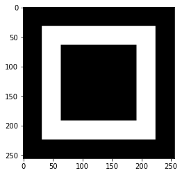
As you can see, it is quite a beauty. It looks the same in 3D since it is a single horizontal slab.
Create a sinogram
A sinogram is created as a result of a forward projection of the volume data. This is the ASTRA way to create a 2D sinogram
# Create a sinogram using the GPU.
# Note that the first time the GPU is accessed, there may be a delay
# of up to 10 seconds for initialization.
proj_id = astra.create_projector('cuda',proj_geom,vol_geom)
sinogram_id, sinogram = astra.create_sino(phantom_2d, proj_id)
A = ts.operator(vg, pg)         # Create forward operator
sino = A(phantom_3d)            # Apply it to the data
plt.subplot(131, title="Phantom")
plt.imshow(phantom_2d)
plt.subplot(132, title="Sinogram ASTRA")
plt.imshow(sinogram)
plt.subplot(133, title="Sinogram tomosipo")
plt.imshow(sino[0])   # pick first (and only) sinogram from 3D stack
plt.show()
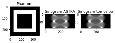
As you can see, the sinograms are exactly the same. This is expected, since tomosipo uses ASTRA under the hood to perform all computations.
Cleaning up
Now for the fun part! For reasons we will not delve into, ASTRA wants to own the data that it operates on. Therefore, you have to tell it that you are done with the data so that it releases it.
astra.data2d.delete(sinogram_id)
astra.projector.delete(proj_id)
In tomosipo, this is not necessary. Since all the data that was created is created using numpy, the Python interpreter can automatically free the memory when dat is not used anymore. To force this, use:
del sino
Summary
To create a sinogram in ASTRA, execute:
import astra
import numpy as np

# Create geometries
vol_geom = astra.create_vol_geom(256, 256)
angles = np.linspace(0,np.pi,180,False)
proj_geom = astra.create_proj_geom('parallel', 1.0, 384, angles)
# Create phantom (code omitted)
phantom_2d = get_phantom()
# Create sinogram
proj_id = astra.create_projector('cuda',proj_geom,vol_geom)
sinogram_id, sinogram = astra.create_sino(P, proj_id)
# Free memory
astra.data2d.delete(sinogram_id)
astra.projector.delete(proj_id)
In tomosipo, the same sinogram can be obtained using:
import tomosipo as ts
import numpy as np

# Create geometries
vg = ts.volume(shape=(1, 256, 256))
pg = ts.parallel(angles=180, shape=(1, 384))
# Create phantom (code omitted)
phantom_3d = get_phantom()
# Create sinogram
A = ts.operator(vg, pg)
sino = A(phantom_3d)
Thanks to Willem Jan Palenstijn for spotting some typos!


