Chambolle-Pock algorithm on the GPU using tomosipo

Jul 30, 2020

Allard Hendriksen

11 minute read

CI
tomosipo

The Chambolle-Pock algorithm, or primal-dual hybrid gradient algorithm, is a convex optimization algorithm. This algorithm can be used to solve the total-variation minimization optimization problem in tomograpy. In this blog post, we follow the exposition by ^{sidky-2012-convex-optim} to obtain a working implementation of PDHG for tomography. We solve the following optimization problems

\begin{align} \label{eq:1} \text{argmin}_{x} &||A x - y ||_2^2 &(\text{Least-squares}) \\\
\text{argmin}_{x} &||A x - y ||_2^2 + \lambda || |\nabla x| ||_1 &(\text{Total-variation minimization}) \end{align}

We are going to skip over all theory, and jump right into the implementation of the algorithms. If you want to know more about proximals, read ^{sidky-2012-convex-optim}.

Setting up the problem

We first import some necessary packages, including PyTorch, and define an auxiliary plotting function:

import numpy as np
import torch
import tomosipo as ts
import tomosipo.torch_support
import matplotlib.pyplot as plt


def plot_imgs(height=3, cmap="gray", clim=(None, None), **kwargs):
    fig, axes = plt.subplots(
        nrows=1,
        ncols=len(kwargs),
        figsize=(height * len(kwargs), height)
    )
    fig.patch.set_alpha(1.0)
    if len(kwargs) == 1:
        axes = [axes]
    for ax, (k, v) in zip(axes, kwargs.items()):
        if isinstance(v, torch.Tensor):
            v = v.cpu().numpy()
        pcm = ax.imshow(v.squeeze(), cmap=cmap, clim=clim)
        fig.colorbar(pcm, ax=ax)
        ax.set_title(k)
    fig.tight_layout()

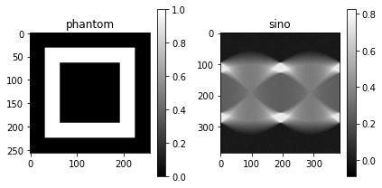
Then we can define a phantom, the venerable hollow box, and create a sinogram:

# Use GPU
dev = torch.device("cuda")

# Create tomosipo geometries
vg = ts.volume(shape=(1, 256, 256), size=(1/256, 1, 1))
pg = ts.parallel(angles=384, shape=(1, 384), size=(1/256, 1.5))
A = ts.operator(vg, pg)

phantom = torch.zeros(A.domain_shape, device=dev)
phantom[:, 32:224, 32:224] = 1.0  # box
phantom[:, 64:192, 64:192] = 0.0  # and hollow

y = A(phantom)
# Add 10% Gaussian noise
y += 0.1 * y.mean() * torch.randn(*y.shape, device=dev)

plot_imgs(
    phantom=phantom,
    sino=y.squeeze().transpose(0, 1)
)

Least-squares

Given the forward operator \(A\) and sinogram \(y\), the Chambolle-Pock algorithm for the least-squares problem is defined as follows:

\(L ← ||A||_2 ; \tau ← 1/L; \sigma ← 1/L; \theta ← 1; n ← 0\)
initialize \(u_0\) and \(p_0\) to zero values;
\(\bar u_0 ← u_0\)
repeat
\(\quad p_{n+1} ← (p_n + \sigma (A \bar u_n − y))/(1 + \sigma )\)
\(\quad u_{n+1} ← u_n − \tau A^T p_{n+1}\)
\(\quad \bar u_{n+1}← u_{n+1} + \tau (u_{n+1} − u_{n} )\)
\(\quad n ← n + 1\)
until \(n \geq N\)

We need an estimate of \(L\), the operator norm of \(A\). This can be computed using power iteration:

def operator_norm(A, num_iter=10):
    x = torch.randn(A.domain_shape)
    for i in range(num_iter):
        x = A.T(A(x))
        x /= torch.norm(x) # L2 vector-norm
    return (torch.norm(A.T(A(x))) / torch.norm(x)).item()

print(operator_norm(A))

1.4483206272125244

Translating the algorithm to Python is quite straight-forward:

L = operator_norm(A, num_iter=100)
t = 1.0 / L                     # τ
s = 1.0 / L                     # σ
theta = 1                       # θ
N = 500                         # Compute 500 iterations

u = torch.zeros(A.domain_shape, device=dev)
p = torch.zeros(A.range_shape, device=dev)
u_avg = torch.clone(u)

residuals = np.zeros(N)
for n in range(N):
    p = (p + s * (A(u_avg) - y)) / (1 + s)
    u_new = u - t * A.T(p)
    u_avg = u_new + theta * (u_new - u)
    u = u_new
    residuals[n] = torch.square(A(u) - y).mean().item()

rec = u.cpu()                   # move final reconstruction to CPU

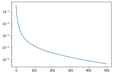
We can plot the residuals:

plt.plot(residuals)
plt.yscale('log')

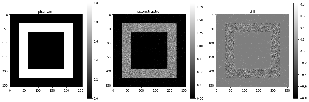
And of course also the resulting reconstruction:

plot_imgs(
    phantom=phantom,
    reconstruction=u,
    diff=u-phantom,
    height=5,
)

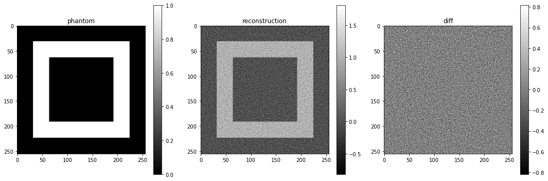It looks a bit noisy.

Least-squares with non-negativity constraint

Adding a non-negativity constraint requires only a single-line change in the algorithm:

L = operator_norm(A, num_iter=100)
t = 1.0 / L                     # τ
s = 1.0 / L                     # σ
theta = 1                       # θ
N = 500                         # Compute 500 iterations

u = torch.zeros(A.domain_shape, device=dev)
p = torch.zeros(A.range_shape, device=dev)
u_avg = torch.clone(u)

residuals_non_neg = np.zeros(N)
for n in range(N):
    p = (p + s * (A(u_avg) - y)) / (1 + s)
    # Add non-negativity constraint
    u_new = torch.clamp(u - t * A.T(p), min=0.0, max=None)
    u_avg = u_new + theta * (u_new - u)
    u = u_new
    residuals_non_neg[n] = torch.square(A(u) - y).mean().item()

rec = u.cpu()                   # move final reconstruction to CPU

We can plot the residuals

plt.plot(residuals, label="without constraint")
plt.plot(residuals_non_neg, label="with non-negativity constraint")
plt.title("Residuals of least-squares")
plt.legend()
plt.yscale('log')

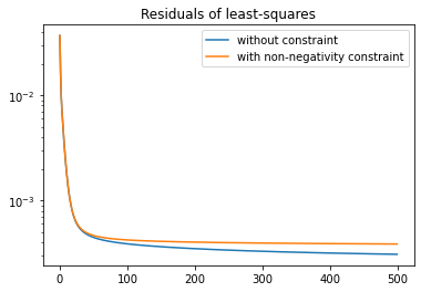
The non-negativity constraint places limits on how closely the reconstruction can fit the data, as we see in the graph above.

In the reconstruction, the background looks a lot better now:

plot_imgs(
    phantom=phantom,
    reconstruction=u,
    diff=u-phantom,
    height=5,
)

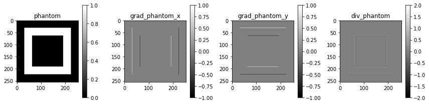
The 2D gradient

To compute the total variation, we must first be able to compute \(\nabla x\), which we call grad_2D in the code below. The transpose of this operation, the negative divergence, we call grad_2D_T. The code below defines the operations, and describes how the operations look when applied to the phantom:

def grad_2D(x):
    weight = x.new_zeros(2, 1, 3, 3)
    weight[0, 0] = torch.tensor([[0, 0, 0], [-1, 1, 0], [0, 0, 0]])
    weight[1, 0] = torch.tensor([[0, -1, 0], [0, 1, 0], [0, 0, 0]])
    x = x[:, None]              # Add channel dimension
    out = torch.conv2d(x, weight, padding=1)
    return out[:, :, :, :]

def grad_2D_T(y):
    weight = y.new_zeros(2, 1, 3, 3)
    weight[0, 0] = torch.tensor([[0, 0, 0], [-1, 1, 0], [0, 0, 0]])
    weight[1, 0] = torch.tensor([[0, -1, 0], [0, 1, 0], [0, 0, 0]])
    out = torch.conv_transpose2d(y, weight, padding=1)
    return out[:, 0, :, :]      # Remove channel dimension

grad_phantom = grad_2D(phantom)
plot_imgs(
    phantom=phantom,
    grad_phantom_x=grad_phantom[0, 0],
    grad_phantom_y=grad_phantom[0, 1],
    div_phantom=grad_2D_T(grad_phantom),
)

To make sure that the two functions are each others' transpose, we test the adjoint property. That is, we want the following equality to hold for all \(x, y\) in the domain and range of \(A\)

\begin{align} \langle x, A^T y \rangle = \langle A x, y \rangle \end{align}

# <x, A.T y> = <A x, y>

x = torch.randn(1, 10, 10, device=dev)
y = torch.randn(1, 2, 10, 10, device=dev)

def inner_product(a, b):
    return torch.dot(a.flatten(), b.flatten())

lhs = inner_product(x, grad_2D_T(y))
rhs = inner_product(grad_2D(x), y)
print("<x, A.T y> = ", lhs.item())
print("<A x, y>   = ", rhs.item())
assert torch.allclose(lhs, rhs)

<x, A.T y> =  17.99624252319336
<A x, y>   =  17.996238708496094

The Chambolle-Pock algorithm for total-variation minimization

For total-variation minimization, the algorithm is defined as follows:

\(L ← ||(A, \nabla)||_2 ; \tau ← 1/L; \sigma ← 1/L; \theta ← 1; n ← 0\)
initialize \(u_0, p_0\), and \(q_0\) to zero values;
\(\bar u_0 ← u_0\)
repeat
\(\quad p_{n+1} ← (p_n + \sigma (A \bar u_n − y))/(1 + \sigma )\)
\(\quad q_{n+1} ← \lambda(q_n + \sigma \nabla \bar u_n)/\text{max}(\lambda \mathbf{1}, |q_n + \sigma\nabla \bar u_n|)\)
\(\quad u_{n+1} ← u_n − \tau A^T p_{n+1} {\color{red}-} \tau \nabla^{T} q_{n+1}\)
\(\quad \bar u_{n+1}← u_{n+1} + \tau (u_{n+1} − u_{n} )\)
\(\quad n ← n + 1\)
until \(n \geq N\)

Here, we deviate a bit from the presentation in ^{sidky-2012-convex-optim}. Specifically, in line 7, \(\tau \nabla^T q_{n+1}\) is subtracted, whereas in the paper \(\tau \text{ div } q_{n+1}\) is added, using the convention that \(\nabla^T \equiv -div\).

Again, we must obtain an estimate of the operator norm:

def operator_norm_plus_grad(A, num_iter=10):
    x = torch.randn(A.domain_shape)
    operator_norm_estimate = 0.0
    for i in range(num_iter):
        y_A = A(x)
        y_TV = grad_2D(x)
        x_new = A.T(y_A) + grad_2D_T(y_TV)
        operator_norm_estimate = torch.norm(x_new) / torch.norm(x)
        x = x_new / torch.norm(x_new)
    return operator_norm_estimate.item()

print(operator_norm_plus_grad(A))

7.578846454620361

In addition, we have the following operation in line 6, which is applied to \(q_n + \sigma \nabla \bar u_n\),

\begin{align} \label{eq:2} \text{clip}_{\lambda}(z) :=\frac{\lambda z}{\text{max}(\lambda \mathbf{1}, |z|)}. \end{align}

This operation has the effect of thresholding the magnitude of the spatial vector \(z\) at each pixel to the value \(\lambda\). Here, \(\mathbf{1}\) denotes a vector containing all ones.

We implement this operation as follows in PyTorch:

def magnitude(z):
    return torch.sqrt(z[:, 0:1] ** 2 + z[:, 1:2] ** 2)

def clip(z, lamb):
    return z * torch.clamp(lamb / magnitude(z), min=None, max=1.0)

Here, we take care to order the multiplications and divisions so that we never divide zero by zero — which yields NaN —, and we never multiply zero by inf. We check that clipping really clips the magnitudes:

z_random = torch.randn(5, 2)

torch.stack(
    (magnitude(z_random), magnitude(clip(z_random, 1.0))),
    dim=2,
)

tensor([[[2.8268, 1.0000]],
        [[0.8896, 0.8896]],
        [[2.4449, 1.0000]],
        [[2.1251, 1.0000]],
        [[0.8660, 0.8660]]])

Now we are able to translate the algorithm to Python:

# Sinogram with 10% Gaussian noise
y = A(phantom)
y += 0.1 * y.mean() * torch.randn(*y.shape, device=dev)
lamb = 0.01                      # λ
N = 1000

L = operator_norm_plus_grad(A, num_iter=100)
t = 1.0 / L
s = 1.0 / L
theta = 1

u = torch.zeros(A.domain_shape, device=dev)
p = torch.zeros(A.range_shape, device=dev)
q = grad_2D(u)                  # contains zeros (and has correct shape)
u_avg = torch.clone(u)

residuals = np.zeros(N)
objectives = np.zeros(N)
for n in range(N):
    p = (p + s * (A(u_avg) - y)) / (1 + s)
    q = clip(q + s * grad_2D(u_avg), lamb)
    u_new = u - (t * A.T(p) + t * grad_2D_T(q))
    u_avg = u_new + theta * (u_new - u)
    u = u_new
    residuals[n] = torch.square(A(u) - y).mean().item()
    objectives[n] = residuals[n] + lamb * magnitude(grad_2D(u)).abs().mean().item()

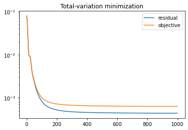
We can plot the residual and objectives as the algorithm progresses:

plt.title("Total-variation minimization")
plt.plot(residuals, label="residual")
plt.plot(objectives, label="objective")
plt.yscale('log')
plt.legend()
plt.show()

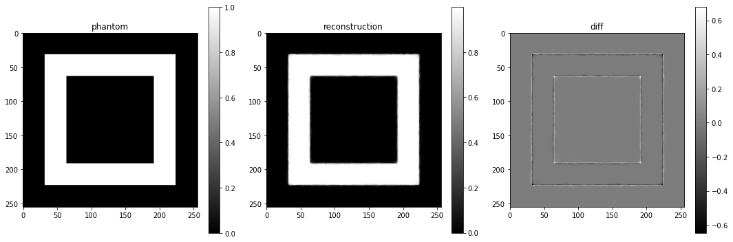
And show the reconstruction, which shows a much improved denoising performance compared to the least-squares solution:

plot_imgs(
    phantom=phantom,
    reconstruction=u,
    diff=u-phantom,
    height=5,
)

Varying the regularization parameter

We define a function that computes the algorithm for arbitrary \(A\) and \(y\). Like before, we can add a non-negativity constraint:

def tv_min_pdhg(A, y, lamb, num_iter=500, L=None, non_negativity=False):
    dev = y.device
    if L is None:
        L = operator_norm_plus_grad(A, num_iter=20)

    t = 1.0 / L
    s = 1.0 / L
    theta = 1

    u = torch.zeros(A.domain_shape, device=dev)
    p = torch.zeros(A.range_shape, device=dev)
    q = grad_2D(u)                       # contains zeros (but has correct shape)
    u_avg = torch.clone(u)

    for n in range(num_iter):
        p = (p + s * (A(u_avg) - y)) / (1 + s)
        q = clip(q + s * grad_2D(u_avg), lamb)
        u_new = u - (t * A.T(p) + t * grad_2D_T(q))
        if non_negativity:
            u_new = torch.clamp(u_new, min=0.0, max=None)
        u_avg = u_new + theta * (u_new - u)
        u = u_new

    return u

Now, we can easily see the effect of the regularization parameter on the hollow box:

L = operator_norm_plus_grad(A, num_iter=20)

reg_params = [1.0, 0.5, 0.1, 1e-2, 1e-5]
plot_imgs(
    phantom=phantom,
    **{f"lambda: {l:0.1e}" : tv_min_pdhg(A, y, l, 500, L=L)
       for l in reg_params}
)

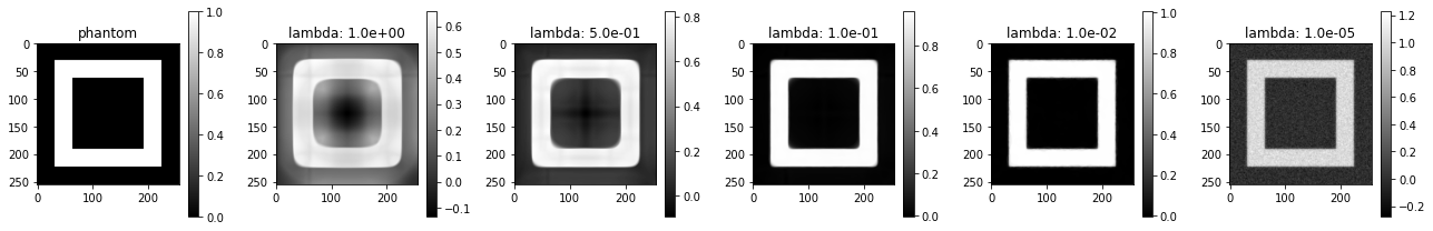
When the regularization parameter is relatively large, TV-normalization appears to introduce rounded corners. When it is small, the noise is not accurately removed anymore.

Speed of computation

We record the time to compute the algorithm using the CPU and on GPU for various number of iterations:

from timeit import default_timer as timer
num_trials = 4
Ns = np.array([1, 2, 4, 8, 16, 32, 64] * num_trials)
times_cuda = np.copy(Ns).astype(np.float32)
times_cpu = np.copy(Ns).astype(np.float32)
for i, N in enumerate(Ns):
    start = timer()
    tv_min_pdhg(A, y.cuda(), 1e-1, N, L=L).cpu()
    times_cuda[i] = timer() - start
    start = timer()
    tv_min_pdhg(A, y.cpu(), 1e-1, N, L=L).cpu()
    times_cpu[i] = timer() - start

We perform a linear fit and plot the result:

# Linear fit:
# https://docs.scipy.org/doc/numpy-1.17.0/reference/generated/numpy.linalg.lstsq.html
W = np.vstack([Ns, np.ones(len(Ns))]).T
a_cuda, b_cuda = np.linalg.lstsq(W, times_cuda, rcond=None)[0]
a_cpu, b_cpu = np.linalg.lstsq(W, times_cpu, rcond=None)[0]

# Plot:
plt.title("Speed of Chambolle-Pock")
plt.plot(Ns, times_cuda, ".", color="blue", label="cuda")
plt.plot(Ns, times_cpu, ".", color="red", label="cpu")
plt.plot(np.arange(max(Ns)), a_cuda * np.arange(max(Ns)) + b_cuda, color="blue")
plt.plot(np.arange(max(Ns)), a_cpu * np.arange(max(Ns)) + b_cpu, color="red")
plt.xlabel("N")
plt.ylabel("Time (s)")
plt.legend()
plt.show()

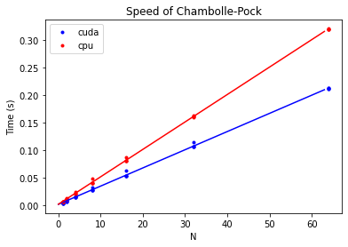
We find that moving all operations to the gpu can be faster:

print(f"Speedup using CUDA: {a_cpu / a_cuda: 0.2f}")

Speedup using CUDA:  1.51

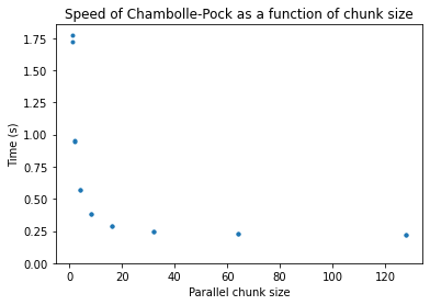
The speedup, however, is slightly disappointing. Perhaps the GPU code is faster when it computes multiple 2D reconstructions in parallel. We test this hypothesis using the following code:

from timeit import default_timer as timer
num_trials = 2
chunk_sizes = np.array(sorted([1, 2, 4, 8, 16, 32, 64, 128] * num_trials))
max_chunk = max(chunk_sizes)
times_chunks = np.copy(chunk_sizes).astype(np.float32)
for i, C in enumerate(chunk_sizes):
    A_chunk = ts.operator(
        vg,
        ts.parallel(angles=384, shape=(C, 384), size=(C/256, 1.5))
    )
    y_chunk = torch.cat((y,) * C)
    start = timer()
    # Always compute max_chunk reconstructions:
    for _ in range(max_chunk // C):
        tv_min_pdhg(A_chunk, y_chunk, 1e-1, 4, L=L).cpu()
    times_chunks[i] = timer() - start

We find that computing multiple reconstructions in parallel can really speed up reconstruction, with diminishing returns at a chunk size of around 64.

# Plot:
plt.title("Speed of Chambolle-Pock as a function of chunk size")
plt.plot(chunk_sizes, times_chunks, ".")
plt.xlabel("Parallel chunk size")
plt.ylabel("Time (s)")
plt.ylim(0, None)
plt.show()

Now, we compare the GPU and CPU code again, at a chunk size of 64:

from timeit import default_timer as timer
C = 64
A_chunk = ts.operator(
    vg,
    ts.parallel(angles=384, shape=(C, 384), size=(C/256, 1.5))
)
y_chunk = torch.cat((y,) * C)

y_chunk = y_chunk.cuda()
start = timer()
tv_min_pdhg(A_chunk, y_chunk, 1e-1, 100, L=L).cpu()
time_cuda = timer() - start

y_chunk = y_chunk.cpu()
start = timer()
tv_min_pdhg(A_chunk, y_chunk, 1e-1, 100, L=L).cpu()
time_cpu = timer() - start

print(f"Speedup using CUDA: {time_cpu / time_cuda: 0.2f}")

Speedup using CUDA:  2.19

We obtain a modest speed improvement this way.

Summary

We have shown how to implement the Chambolle-Pock algorithm on the GPU using tomosipo and PyTorch. The Python implementation follows the listed algorithm quite closely, and computation of the gradient is simplified and fast because it can be expressed as a convolution, which happens to be a fast operation in deep learning frameworks such as PyTorch. In addition, we show that performing all computations on the GPU can be faster than on CPU, and that computing multiple reconstructions in parallel can improve throughput even more.

Thanks to Rien Lagerwerf for valuable comments that improved this post, and to Francien Bossema, who spotted various errors!

Allard Hendriksen | CI @ CWI